AGGREGATE DEMAND AND AGGREGATE SUPPLY
What goes on in the aggregate goods and services market is vital to the health of an economy. Indeed, if we could keep our eye on just one market in an economy, we would choose the goods and services market, since it exerts a vital impact on our economic opportunity and standard of living. It is important to note that the quantity and price variables in this highly aggregated market differ from their counterparts in the market for a specific good. The quantity variable in the aggregate goods and services market is real GDP--the flow of goods and services produced and purchased during a period. The price variable in the goods and services market represents the average price of goods and services purchased during the period. In essence, it is the economy's price level, as measured by a general price index (for example, the GDP deflator).
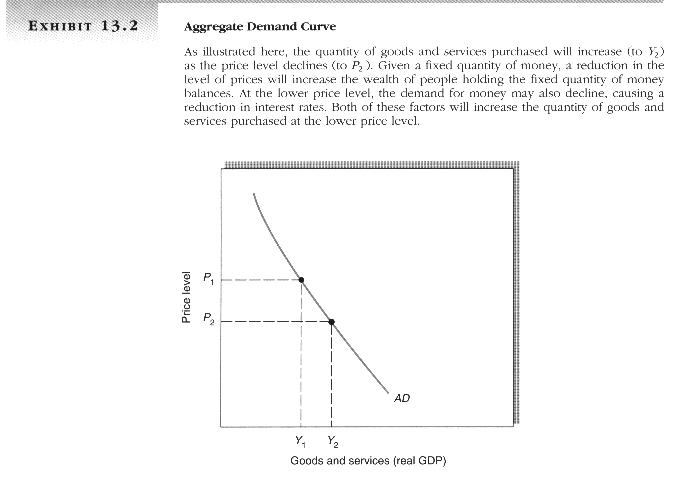
Aggregate Demand
Just as the concepts of demand and supply enhance our understanding of markets for specific goods, they also contribute to our understanding of a highly aggregated market such as that for goods and services. The purchases of consumers, investors, governments, and foreigners comprise the nation's demand for goods and services. Thc aggregate demand curve indicates the various quantities of goods and services that purchasers are willing to buy at different price levels. As Exhibit 13.2 illustrates, the aggregate demand curve (AD) is a downward-sloping schedule, indicating that as the price level declines, people are willing to purchase more and more output. Alternatively, the quantity of goods and services purchased declines as the price level rises.
The explanation of the downward-sloping aggregate demand schedule differs from that for a specific commodity. The inverse relationship between price and the amount demanded of a specific commodity, TV sets, for example, reflects the fact that consumers turn to substitutes when a price increase makes a good more expensive. This relative price change will not be present when there is a change in the price of all goods. Instead, the inverse relationship between the price level and aggregate amount demanded reflects the impact of the fixed quantity of money. As the level of prices declines, the purchasing power of the fixed quantity of money increases. For example, if you have $2,000 in your bank account, your wealth would increase if there was a 25 percent reduction in the price of goods and services. At the lower price level, your $2,000 will buy more goods and services. Other people are in an identical position. As the price level declines, the purchasing power of their money balances also increases. This increase in wealth derived from the expansion in the purchasing power of the fixed money balances will induce people to purchase more goods and services as the price level declines. In addition, a lower price level may also reduce the amount of money households and businesses want to hold in order to make purchases and conduct their affairs. The decline in the demand for money relative to the fixed supply of money will place downward pressure of interest rates. This, too, will encourage people to purchase more goods and services. Therefore, even though the explanation differs, the aggregate demand curve, like the demand curve for a specific product, slopes downward to the right.
Aggregate Supply
In view of the preceding discussion, it should come as no great surprise to the reader that the explanation for the general shape of the aggregate supply curve also differs from that for the supply curve of a specific good. When considering aggregate supply, it is particularly important to distinguish between the short run and the long run. In this context, the short run is the time period during which some prices, particularly those in labor markets, are set by prior contracts and agreements. Therefore, in the short run, households and businesses are unable to adjust these prices in light of unexpected recent changes, including unexpected changes in the price level. In contrast, the long run is a time period of sufficient duration that people have the opportunity to learn more fully about recent price changes and to modify their prior choices in response to them. We now consider both the short-run and long-run aggregate supply curves (Exhibit 13.3).
SHORT-RUN AGGREGATE SUPPLY The short-run aggregate supply; (SRAS) curve indicates the various quantities of goods and services that firms will supply at different price levels during the period immediately following a change in the price level. As Exhibit 13.3a illustrates, the 5RAS curve slopes upward to the right, reflecting the fact that in the short run an unexpected increase in the price level will improve the profitability of firms, and they will respond with an expansion in output.
The SRAS curve is based on a specific expected price level, P100 in the case of Exhibit 13.3. When that price level is achieved, firms will earn normal profits and supply output Y0. Why will an increase in the price level (to P105, for example) enhance profitability, at least in the short run? Profit per unit equals price minus the producer's per unit costs. Important components of producers' costs will be determined by long-term contracts. Interest rates on loans, collective bargaining agreements with employees, lease agreements on buildings and machines, and other contracts with resource suppliers will influence production costs during the current period. The prices incorporated into these long-term contracts at the time of the agreement are based on the expectation of price level (P~00) for the current period. These resource costs tend to be temporarily fixed. If an increase in demand causes the price level to rise unexpectedly during the current period, prices of goods and services will increase relative to the temporarily fixed components of costs. Profit margins will improve, and business firms will happily respond with an expansion in output (to Y1).
An unexpected reduction in the price level to P95 would exert just the opposite effects. It would decrease product prices relative to costs and thereby reduce profitability. In response, firms would reduce output to Y2. Therefore, in the short run, there will be a direct relationship between amount supplied and the price level in the goods and services market.
LONG-RUN AGGREGATE SUPPLY The long-run aggregate supply (LRAS) curve indicates thc relationship between the price level and quantity of output after decision makers have had sufficient time to adjust their prior commitments in light of any previously unexpected changes in market prices. A higher price level in the goods and services market will fail to alter the relationship between production and resource prices in the long run. Once people have time to adjust fully their prior commitments, competitive forces will restore the usual relationship between product prices and costs, Profit rates will return to normal, removing the incentive of firms to supply a larger rate of output. Therefore, as Exhibit 13.3b illustrates, the LRAS curve is vertical.
The forces that provided for an upward-sloping SRAS curve are absent in the long run. Costs that are temporarily fixed due to long-term contracts will eventually rise. With time, the long-term contracts will expire and be renegotiated. Once the contracts are renegotiated, resource prices will increase in the same proportion as product prices. A proportional increase in costs and product prices will leave the incentive to produce unchanged. Consider how a firm with a selling price of $20 and per unit costs of $20 will be affected by the doubling of both product and resource prices. After the price increase, the firm's sales price will be $40, but so, too, will its per unit costs. Thus, neither the firm's profit rate nor the incentive to produce is changed. Therefore, in the long run an increase in the nominal value of the price level will fail to exert a lasting impact on aggregate output.
Reflecting on the production possibilities of an economy also sheds light on why the long-run aggregate supply curve is vertical. As we discussed in Chapter 1, at a point in time, our production possibilities are constrained by the supply of resources, level of technology, and institutional arrangements that influence the efficiency of resource use. A higher price level does not loosen these constraints. For example, a doubling of prices will not improve technology. Neither will it expand the availability of productive resources (once expectations have adjusted to the change) nor improve the efficiency of our economic institutions. Thus, there is no reason for a higher price level to increase our ability to produce goods and services. This is precisely what the vertical LRAS curve implies. The accompanying "Thumbnail Sketch" summarizes the factors that explain the general characteristics of aggregate demand, short-run aggregate supply, and long-run aggregate supply.